


Setting up the first dropdown list
There are three default options, hence, you can fix these values for the first dropdown list.
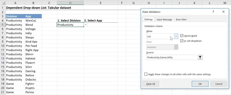
Select the cell (D5).
Go to Data > Data Validation.
Under the Validation criteria:
- Allow: List
- Source: Productivity, Game, Utility
Featured Bundle
Black Belt Excel Bundle

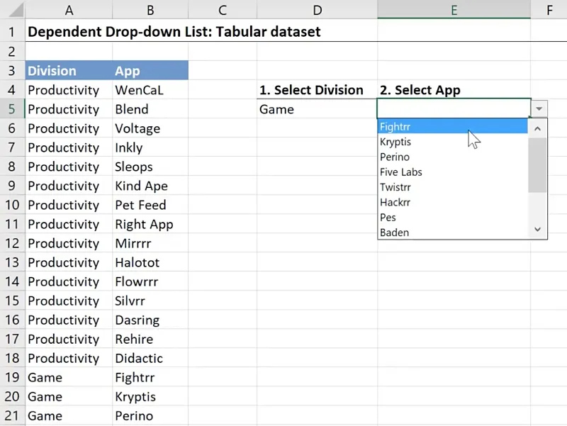
Setting up the second dropdown list
Since this will be dependent on the selected option of the first dropdown list, the values should not be fixed.
Instead, we can use MS Excel’s OFFSET() function to find the corresponding list. (Here is a link to a separate guide to the basics of the OFFSET() function.)
This function works similar to a GPS.
Unlike INDEX(), it doesn’t need a predefined map with regards to where it should move.
All you have to do is provide it with a starting point and it can move to any direction from that point.
The syntax for the OFFSET() function is:
= OFFSET(reference, rows, cols, [height], [width])- reference: This is the starting point. It makes sense to use a cell which is close to the answer. Since the list options that we want to display are found in column B, we use cell B3 as the starting point. Any cell can be used as the starting point as long as you take note that the arguments will change depend on the chosen starting point.
- rows: This defines how many rows down you want to move. In this case, it depends on the selected option of the first dropdown list. You would want to move down up until the first occurrence of the Division. The MATCH() function is a good fit, where you lookup the division and match it with your source table.
Here we use: MATCH(D5,A4:A43,0). A quick way to highlight up until the last cell of the table is to hold CTRL + SHIFT + ¯.
- cols: This defines how many columns you want to move to find the answer. Since the answer is in column B and the starting point is also in column B, there is no need to move columns. Hence, 0 is used.
- [height]: This defines how many rows you want to return. Placing a 1 means that the formula returns 1 value. In this case, we want to count how many cells of data there are a specific Division. To do this, the COUNTIF() function can be used. There are two parameters for this: the range (the division column, cells A4:A43) and the criteria (the Division, cell D5).
We write it as COUNTIF(A4:A43,D5).
- [width]: An optional argument that counts how many columns you want to return. In this case we want it to be 1.
The final formula becomes:
= OFFSET(B3,MATCH(D5,A4:A43,0),0,COUNTIF(A4:A43,D5), 1)This will seem to result in an error but only because Excel can’t put all the results in a single cell. What you can do to check if the correct values are returned is to go to the formula bar, highlight the formula and press F9. This should display the values. Countercheck if this includes up until the last App under that Division.

Make sure to fix the cell references:
= OFFSET($B$3,MATCH($D$5,$A$4:$A$43,0),0,COUNTIF($A$4:$A$43,$D$5), 1)All that’s left to do is to copy the final formula and use it as the source for the second dropdown list.
Select the cell where you want to place the second dropdown list (cell E5).
Go to Data > Data Validation.
Under Allow, select List.
Paste the formula as the Source.

This should now create a second dropdown list which is dependent on the Division selected.
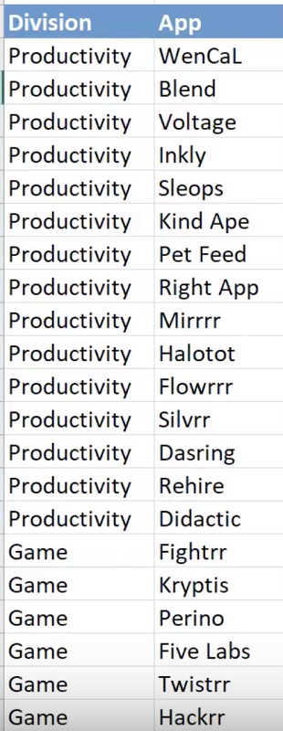
An important thing to note is that your Divisions should be grouped together.
You can easily do this by sorting out the values of the Division column after adding a new App.
Feel free to Download the Workbook HERE.


Leila Gharani
I’ve spent over 20 years helping businesses use data to improve their results. I've worked as an economist and a consultant. I spent 12 years in corporate roles across finance, operations, and IT—managing SAP and Oracle projects.
As a 7-time Microsoft MVP, I have deep knowledge of tools like Excel and Power BI.
I love making complex tech topics easy to understand. There’s nothing better than helping someone realize they can do it themselves. I’m always learning new things too and finding better ways to help others succeed.


