Excel VSTACK Function – Combine Data from Multiple Sheets

Download the practice workbook 👉 HERE and follow along.

Do you have data scattered across multiple sheets in Excel? Combining this information can be tedious. Fortunately, Excel’s VSTACK function simplifies this task.

What is the VSTACK Excel Function?

VSTACK is a function in Excel that stacks arrays vertically. It allows you to combine data from different ranges or sheets into a single column.

This is really useful when you’re trying to keep all your information in one place.

How to Use Excel VSTACK

The syntax for VSTACK is straightforward:

=VSTACK(array1, [array2], ...)

• array1: The first range of data you want to stack.
• [array2], …: Additional ranges to include in the stack.

Each array represents a set of data. VSTACK combines these arrays into one continuous column.

Featured Course

Master Excel’s Essential Modern Functions

Master the essential Excel functions most professionals don’t know: FILTER, SORT, UNIQUE, XLOOKUP, SEQUENCE. Create reports in minutes instead of hours.

Learn More

Combine Data from Multiple Sheets in Excel

Do you have several sheets with similar tables in Excel? Here’s how you can combine all the data into one table using the VSTACK function.

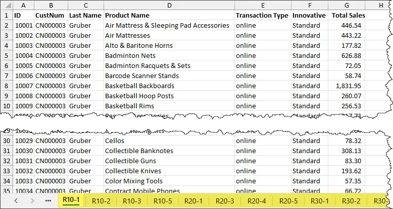
Step-by-Step Instructions

1. Create a Consolidated Sheet:

• Open a new sheet and name it “ConsolidatedData.”

2. Add Headers:

• In cell A1, type the column headers from one of your tables.

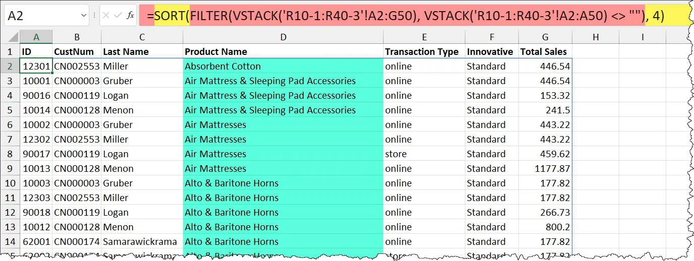
3. Enter the VSTACK Formula:

• In cell A2, enter this formula:

=VSTACK('R10-1:R40-3'!A2:G50)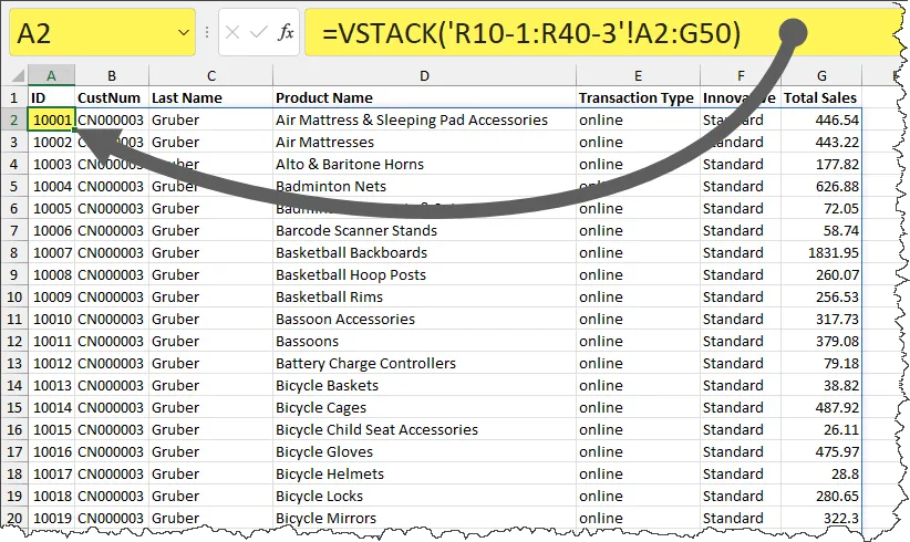

💡 Tip: The sheet names “R10-1” and “R40-3” act as bookends. Any sheets placed between these two will be included in the formula. This is called a 3D Range Reference.

4. Understand the Output:

• The formula stacks all data from the range A2in every sheet between “R10-1” and “R40-3.”
• You’ll get a single table combining all the rows.

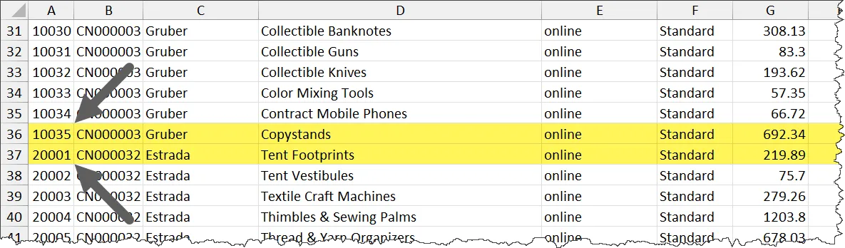
Handling Blank Rows

When you use the VSTACK function, you might see rows filled with zeros where there’s no data.

These rows aren’t actual data—they’re placeholders for empty cells.

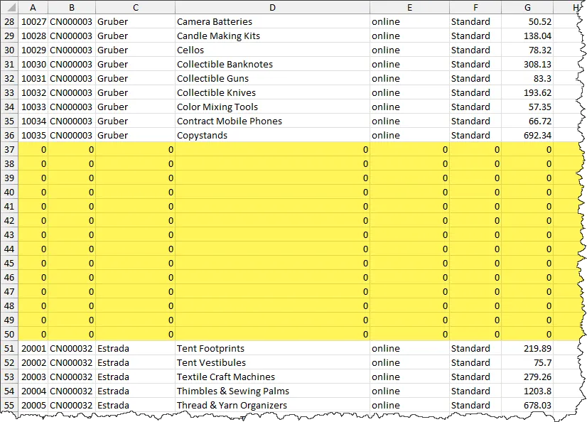
Let’s fix that by using the Excel FILTER function.

=FILTER(VSTACK('R10-1:R40-3'!A2:G50), VSTACK('R10-1:R40-3'!A2:A50) <> "")

What This Formula Does:

• FILTER Function: Filters out rows where column A is empty.
• VSTACK in the Include Argument: Checks if column A has any data (<> "") to decide which rows to keep.

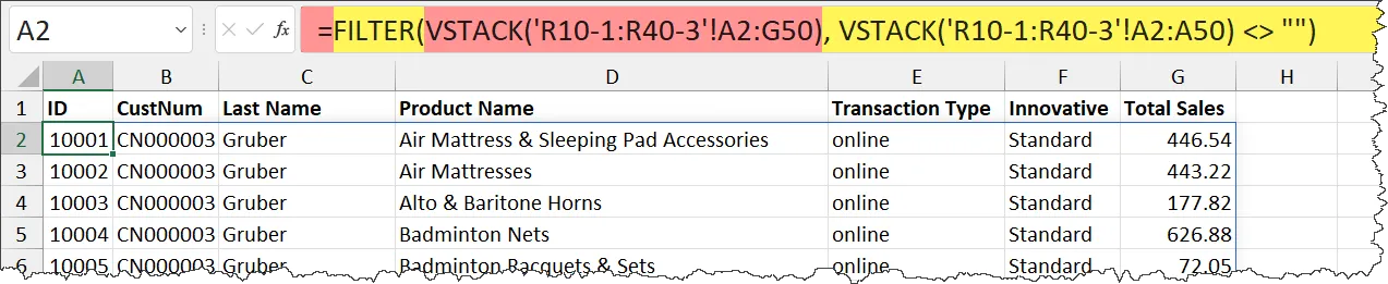
After applying the FILTER formula, your table will exclude all blank rows.

The final output will include only rows with actual data.

Discover how to use the Excel FILTER function with step-by-step examples in our detailed article.

Featured Bundle

Power Excel Bundle

10x your productivity in Excel 💪 by mastering Excel’s Power Tools in ONE convenient (cost savings) bundle. Learnings apply to Power BI as well.

Learn More

How to Sort Filtered and Stacked Results in Excel

Once you’ve combined and cleaned your data using VSTACK and FILTER, you might need to sort the results.

Whether it’s by product name or sales figures, Excel’s SORT function makes it easy.

Step 1: Sorting by a Single Column

Here’s how to sort your data by a single column, like “Product Name”:

Enter this formula in your sheet:

=SORT(FILTER(VSTACK('R10-1:R40-3'!A2:G50), VSTACK('R10-1:R40-3'!A2:A50) <> ""), 4)

• FILTER Function: Removes blank rows from the stacked data.
• SORT Function: Sorts the data by the 4th column (e.g., “Product Name”).

• The number 4 in the formula is the sort_index. It tells Excel to sort by the 4th column in the range.
• By default, the SORT function arranges data in ascending order.

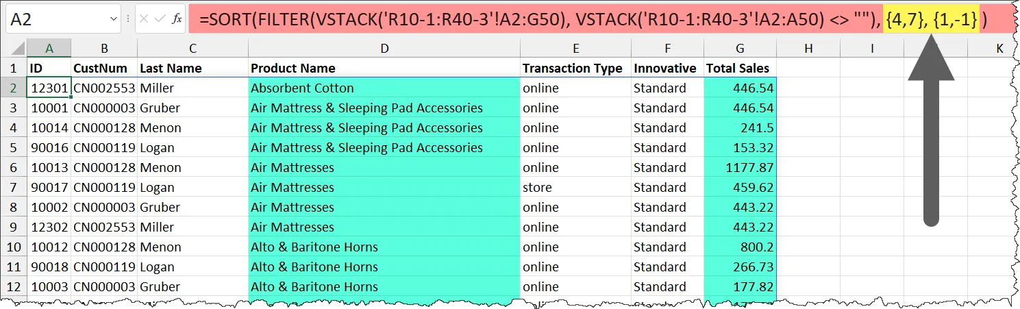
Step 2: Multi-Level Sorting

Need to sort by more than one column? For example, “Total Sales” within each “Product Name”?

Use this modified formula:

=SORT(FILTER(VSTACK('R10-1:R40-3'!A2:G50), VSTACK('R10-1:R40-3'!A2:A50) <> ""), {4,7}, {1,-1} )

Here’s what it does:

1. Primary Sort (Column 4):
   • {4,7} tells Excel to sort first by the 4th column (“Product Name”).
   • 1 specifies ascending order for this column.
2. Secondary Sort (Column 7):
   • Excel then sorts by the 7th column (“Total Sales”).
   • -1 specifies descending order for this column.

Understanding the Curly-Braces

If curly braces {} are new to you, here’s a simple explanation:

• Curly braces allow Excel to handle multiple inputs at once.
• In this formula:
  • {4,7} lists the columns to sort by (4th and 7th columns).
  • {1,-1} specifies the sort direction for each column (ascending for column 4, descending for column 7).

Formatting the Output

By default, Excel does not carry over cell formatting from the original data to the VSTACK output.

Here’s how to fix this:

1. Manually Apply Formatting:
   • After creating your VSTACK formula, select the output range.
   • Go to the Home tab and use the Format Cells option to apply the same styles as your source data.
2. Use Conditional Formatting (Optional):
   • If your source data had conditional formatting, you can replicate it in the output by applying the same rules in the Conditional Formatting menu.

💡 Learn more about conditional formatting in our detailed article.

Avoiding Circular Reference Errors

If you’re combining data within the same workbook, be careful where you place the output sheet. Here’s why:

The Problem:
If your output sheet is included in the range of sheets used in your VSTACK formula, Excel will create a circular reference error.

This happens because the formula tries to reference its own results, creating an endless loop.

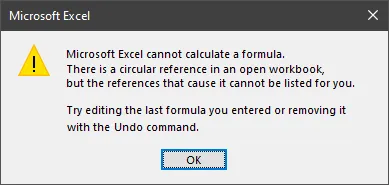
The Solution:

Always place the output sheet outside the range of sheets being stacked.

For example, if your formula references sheets “Sheet1” to “Sheet3,” place the output on a new sheet named “ConsolidatedData” outside this range.

How to Dynamically Include New Sheets

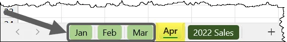
If you’re combining data from multiple sheets with Excel’s VSTACK function, adding a new sheet (like “Apr” for a new month) can break your formula.

Let’s explore how to fix this issue without constantly updating the formula.

The Problem: Adding New Sheets

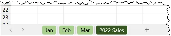
Imagine you’re combining data from sheets named “Jan,” “Feb,” and “Mar” using this formula:

=VSTACK(Jan:Mar!A2:B50)

If you add a new sheet called “Apr,” Excel won’t include it in the VSTACK results because it falls outside the defined range (Jan:Mar).

This means you’ll have to update the formula every time you add a new sheet.

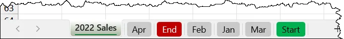
The Solution: Use Bookend Sheets

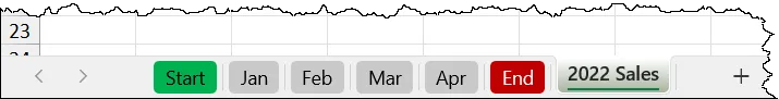
A better way to handle this is by creating permanent bookend sheets called “Start” and “End.”

These sheets act as placeholders, and any new sheet added between them is automatically included in the VSTACK formula. Here’s how to set it up:

1. Create Bookend Sheets:
Add two blank sheets named “Start” and “End.”

Place them before and after all the sheets you want to include in your formula.

2. Update the Formula:
Rewrite your VSTACK formula to reference the bookend sheets:

=VSTACK(Start:End!A2:B50)

3. Add New Sheets:
When adding a new sheet (e.g., “Apr”), place it between the “Start” and “End” sheets.

It will automatically be included in the results.

4. Removing Blank Rows from Bookend Sheets

Since the “Start” and “End” sheets don’t have data, they’ll introduce blank rows into your VSTACK output.

Use the FILTER function to clean up the results:

=FILTER(VSTACK(Start:End!A2:B50), VSTACK(Start:End!A2:A50) <> "")

Featured Course

Excel Pivot Tables & Dashboards

Learn to build Pivot Tables that summarize thousands of rows instantly. Create interactive dashboards that update themselves. No manual sorting or complicated formulas needed.

Learn More

How to Automatically Sort Sheets with VBA

When using bookend sheets like “Start” and “End” for your VSTACK formula, it’s essential to ensure that all new sheets fall between them.

Instead of manually rearranging sheets, you can use VBA (Visual Basic for Applications) to sort them automatically.

Before You Start

To use VBA, you need to save your Excel workbook as a macro-enabled file (.XLSM). Here’s how:

1. Go to File > Save As.
2. In the “Save as type” dropdown, select Excel Macro-Enabled Workbook (*.xlsm).
3. Click Save.

Step 1: Open the Visual Basic Editor

1. Use the keyboard shortcut Alt + F11 to open the Visual Basic Editor.
2. In the editor, go to Insert > Module.
3. A blank module sheet will appear.

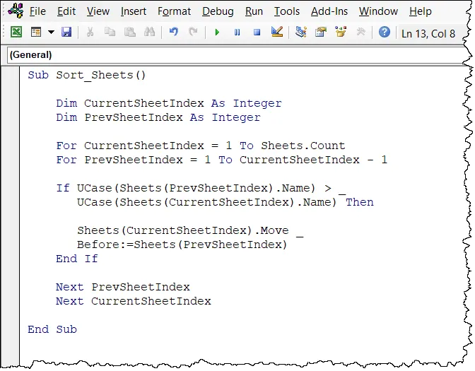
Step 2: Add the VBA Code

Copy and paste the following code into the module sheet:

Sub Sort_Sheets()
  Dim CurrentSheetIndex As Integer
  Dim PrevSheetIndex As Integer
  For CurrentSheetIndex = 1 To Sheets.Count
    For PrevSheetIndex = 1 To CurrentSheetIndex - 1
      If UCase(Sheets(PrevSheetIndex).Name) > _
      UCase(Sheets(CurrentSheetIndex).Name) Then
        Sheets(CurrentSheetIndex).Move _
        Before:=Sheets(PrevSheetIndex)
      End If
    Next PrevSheetIndex
  Next CurrentSheetIndex
End Sub

Step 3: Run the Code

1. Close the Visual Basic Editor by pressing Alt + Q.
2. Back in Excel, press Alt + F8 to open the Macro dialog box.
3. Select Sort_Sheets from the list and click Run.

The macro will sort your sheets alphabetically, ensuring that any new sheets fall between “Start” and “End.”

Featured Course

Unlock Excel VBA & Excel Macros

Automate ANYTHING you need done in Excel with VBA and macros. Go from Beginner to VBA Expert and design automations with confidence.

Learn More

Advanced Sheet Sorting in Excel

The problem with this code is that it sorts alphabetically in ascending order. 

Since our sheet tabs have month name abbreviations as well as the bookend names, we will get an undesirable sort result.

You can take sorting to the next level by renaming your sheets. This method ensures they are sorted logically, even when new sheets are added.

Step 1: Understand the Naming Convention

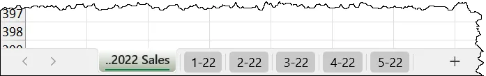
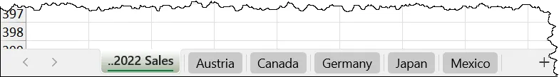
To sort sheets in a meaningful order, we use specific characters that Excel recognizes for sorting:

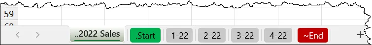
• Periods (.): Sheets starting with a period are sorted before those starting with letters or numbers.
  • Two periods (..): Sorts before one period.
  • Example: ..2022 Sales will appear before .Start.
• Tilde (~): Sheets starting with a tilde are sorted last.
  • Example: ~End will always appear after all other sheets.
• M-YY Format: Using month numbers (e.g., “3-22” for March 2022) forces chronological sorting.

Step 2: Rename Sheets for Proper Sorting

Here’s how to rename your sheets to ensure logical order:

1. Rename month sheets using month number and year:
   • Example: Change Jan to 1-22, Feb to 2-22, and so on.
2. Add special characters to bookend sheets:
   • Rename Start to .Start.
   • Rename End to ~End.
3. Use double periods for key sheets:
   • Rename 2022 Sales to ..2022 Sales.

Step 3: Update the VSTACK Formula

After renaming your sheets, update your VSTACK formula to reflect the new names.

Use single quotes to handle special characters in sheet names:

=VSTACK('.Start:~End'!A2:G50)

Step 4: Run the Sorting Macro

Once the sheets are renamed, you can sort them alphabetically to maintain the desired order:

1. Open the Visual Basic Editor (press Alt + F11).
2. Use the sorting macro provided above.
3. Save your workbook as a macro-enabled file (.XLSM).
4. Run the macro (press Alt + F8 and select Sort_Sheets).

Bonus Tip: Hide Bookend Sheets

To keep your workbook tidy, you can hide the .Start and ~End sheets:

1. Right-click the .Start or ~End tab.
2. Select Hide.

These sheets will remain functional but won’t be visible to users.

Availability

The Excel VSTACK Function is available in Excel for Microsoft 365 and in Excel for the web.

Practice Hands-On with Our Free Workbook

Want to master the Excel VSTACK function quickly? Download our interactive workbook!

What’s Inside:

• Step-by-step example of the VSTACK function in action.
• Practical exercises to reinforce your learning.
• Real-world scenarios to help you apply VSTACK effectively in your work.

Get Started Today:
Click here to download the workbook and follow along as you learn. By practicing these techniques in Excel, you’ll gain the confidence to combine data like a pro.

Featured Bundle

Black Belt Excel Bundle

This Excel Black Belt Package includes EIGHT of our Popular Courses. You’ll learn high-value, in-depth Excel skills that solve real problems.

Learn More

LinkedIn Twitter YouTube

Leila Gharani

I’ve spent over 20 years helping businesses use data to improve their results. I've worked as an economist and a consultant. I spent 12 years in corporate roles across finance, operations, and IT—managing SAP and Oracle projects.

As a 7-time Microsoft MVP, I have deep knowledge of tools like Excel and Power BI.

I love making complex tech topics easy to understand. There’s nothing better than helping someone realize they can do it themselves. I’m always learning new things too and finding better ways to help others succeed.

More About Leila Join 400,000+ professionals in our courses