


Download the practice workbook 👉 HERE and follow along.
Let’s say you have a main Excel sheet called “Summary.” This sheet helps you look at specific information from other sheets within the same file.
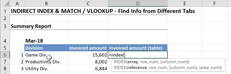
For example, you might want to see invoiced amounts from different departments. These include the Game, Productivity, and Utility divisions.
In addition, you want to have the option to choose a month.

Here’s how you can set it up simply:
The “Summary” sheet includes a cell (B4) where you select a month.
Each division has its own sheet named accordingly: Game Div., Productivity Div., and Utility Div.
These division sheets are organized the same way. They list invoiced amounts month by month.
Your goal is to lookup the invoiced amounts from the relevant division sheet based on the month you’ve selected in the Summary sheet. This setup allows you to view specific financial details quickly and easily.

Why not use the IF Function for a Lookup Across Multiple Sheets
The IF function can help you lookup data from specific tabs based on conditions you set. For example, if you’re looking at divisional data, you might set up the function to get information from the “Game Div” tab when the division is “Game Div,” and similarly for other divisions.
However, this method has a drawback. Every time you add a new tab, you need to update all the IF statements in your summary sheet. This can become cumbersome and prone to errors as your Excel file grows.
A better approach would be to use a formula that automatically adjusts to include any new tabs you add. This makes your Excel sheet easier to manage and more dynamic, accommodating changes without needing constant updates.
Option 1: VLOOKUP Multiple Sheets
To manage data from multiple sheets effectively, you can start with the basic VLOOKUP formula.
Once the basic formula is set up, we will cover how to do a VLOOKUP between two sheets. Learn more about VLOOKUP in this detailed guide.
Setting Up Your Basic Formula:
- Begin in cell C6.
- Use this basic syntax for VLOOKUP:
= VLOOKUP(lookup_value, table_array, col_index_num, [range_lookup])- lookup_value: This is what you’re searching for. For example, the month is listed in cell B4. Make sure to fix this reference to avoid changes as you move the formula around: use $B$4.
- table_array: This is where you find the data. Start with the Game Division tab like this: Game Div.!$A$4:$B$24.
- col_index_num: Choose the column number that has the data you need; here it’s 2 for the second column.
- range_lookup: Set this to FALSE to ensure you only get exact matches.
Example formula for cell C6:
- lookup_value: Since you know that you will be looking at the Game Div. tab, this does not need to be an argument. Lookup value is the cell containing the month, cell B4. Since you want to be able to pull this formula down, fix this cell reference to $B$4.
- table_array: Go to Game Div. and highlight the entire table and add a few more rows to include future data (‘Game Div.’!$A$4:$B$24)
- col_index_num: This tells which column to look at. In this case, since we want the second column in the table array area, we use 2.
- range_lookup: Select TRUE for an approximate match or false for an exact match. In this example, we want an exact match.
= VLOOKUP($B$4, 'Game Div.'!$A$4:$B$24, 2, FALSE)
Making Your Formula Dynamic:
If you copy the formula to different rows, you’ll want it to pull data from various division sheets, not just from one. Let’s look at a VLOOKUP example between two sheets.
The INDIRECT function is perfect for this. It allows you to use text as a reference in your formulas.
Using INDIRECT to Switch Sheets Dynamically:
Purpose of INDIRECT: It converts text into a usable Excel reference. For instance, if you write the division name in a cell, INDIRECT can use that cell’s text to refer to a specific sheet.
How to Use INDIRECT:
- Say cell B6 contains the name of the division, like “Game Div.”.
- Normally, your VLOOKUP formula looks directly at a specific sheet:
= VLOOKUP($B$4, 'Game Div.'!$A$4:$B$24, 2, FALSE)
- To make it dynamic, use INDIRECT to tell Excel to get the sheet name from cell B6 instead of it being fixed in the formula.
Dynamic VLOOKUP Formula:
= VLOOKUP($B$4, INDIRECT("'" & B6 & "'!$A$4:$B$24"), 2, FALSE)Here’s what’s happening:
- INDIRECT(“‘” & B6 & “‘!$A$4:$B$24”) is the key part. It builds the sheet reference from the text in B6.
- ‘&’ connects pieces of text in Excel, making a complete reference that VLOOKUP can use.
- $B$4 is the cell with the month you’re looking up.
- 2 tells VLOOKUP to look in the second column for the amount.
- FALSE specifies you need an exact match.
Now, whenever you change the division name in B6, the formula automatically updates to pull data from the new division’s sheet.
Just copy this formula down the rows, and it will work for any division listed in column B.

If you want to learn more about how the INDIRECT function can make your Excel work more flexible and powerful, feel free to check out our detailed article.
Option 2: INDEX MATCH Across Multiple Sheets
Another option is to use INDEX MATCH for a lookup across multiple sheets. This approach involves converting all the data in the Division tabs into Excel data tables.
Convert Data into Excel Tables:
- Click on any data cell in a Division tab.
- Press CTRL + T to bring up the Create Table window.
- Confirm the data range and click OK to convert the data into an Excel table.

- Rename the table to avoid spaces, like changing “Game Div” to “Game_Div”. This makes referring to them in formulas easier.

Change Table Design (Optional):
- Click on any cell in your newly created table.
- Navigate to the Design tab, choose Table Styles to change its look, or Clear to revert to the original style.

Using INDEX-MATCH to Lookup Data across multiple sheets
Set Up Basic Formula:
Begin with the INDEX function:
= INDEX(array, row_num, [column_num])- array: This is where your data is. For example, “Game_Div.[Invoiced Amount]”.
- row_num: Use the MATCH function here to find the right row. It searches for a specific date in the “Game_Div.[Date]” column and returns its position.
Combine INDEX with MATCH:
The MATCH function looks like this:
= MATCH(lookup_value, lookup_array, [match_type])- lookup_value: This is what you’re searching for, e.g., a date in cell B4 on the Summary tab.
- lookup_array: The column that contains data to match the lookup value, like “Game_Div.[Date]”.
- match_type: Set this to 0 for an exact match.
Example Formula for One Sheet:
= INDEX(Game_Div.[Invoiced Amount], MATCH(Summary!$B$4, Game_Div.[Date], 0))
Making the INDEX MATCH Formula Dynamic Across Sheets:
Dragging this formula down to the Utility Div. row will return the same values since they are hard-coded to look inside the Game Div. tab.
To fix this, we will use the INDIRECT function to help us get the dynamic tab names.
Dynamic Sheet Names with INDIRECT:
- Use INDIRECT to refer dynamically to different division tables based on cell B6 content.
- Replace spaces in names with underscores using the SUBSTITUTE function:
This is the syntax for SUBSTITUTE:
= SUBSTITUTE(text, old_text, new_text, [instance_num]).- text: The cell you want the substitution to take place.
- old_text: What specific character you want to replace. In this case, it is “ “.
- new_text: What to substitute the old_text with. In this case, it is “_”.
- Instance_num: How many times we want the substitution to take place. This is an optional argument. We can leave it out which means we’d like all instances of “ “ to be replace with “_”.
In our case we just need to replace the spaces with and underscore: for example “Game Div” becomes “Game_Div” to match the Excel table name.
= SUBSTITUTE(B6, " ", "_")Full Dynamic Formula:
= INDEX(INDIRECT(SUBSTITUTE(B6, " ", "") & "[Invoiced Amount]"), MATCH(Summary!$B$4, INDIRECT(SUBSTITUTE(B6, " ", "") & "[Date]"), 0))
Drag this formula down from cell D6 to D8 to apply it for other divisions.

If you want a deeper understanding of how to use the INDEX MATCH functions, check out our detailed guide.
With these two methods, you can automatically lookup across multiple sheets. One version used VLOOKUP with cell references and sheet names. The second method used INDEX MATCH with table names.
Download the Workbook
Enhance your learning experience by downloading our workbook. Practice the techniques discussed in real-time and master the INDEX MATCH functions in Excel with hands-on examples.
Download the workbook here and start applying what you’ve learned directly in Excel.

Featured Bundle
Black Belt Excel Bundle


Leila Gharani
I’ve spent over 20 years helping businesses use data to improve their results. I've worked as an economist and a consultant. I spent 12 years in corporate roles across finance, operations, and IT—managing SAP and Oracle projects.
As a 7-time Microsoft MVP, I have deep knowledge of tools like Excel and Power BI.
I love making complex tech topics easy to understand. There’s nothing better than helping someone realize they can do it themselves. I’m always learning new things too and finding better ways to help others succeed.


