


Typical Use of Conditional Formatting
For most users, Conditional Formatting is used to draw attention to cells where the cell’s value meets a defined criterion, such as “greater than 80,000”.

The issue with this method is that if you want to adjust the rule’s values, you must manually update the Conditional Formatting rule.
Conditional Formatting Based on Cell Values
Imagine letting the user type a value into a cell above the data. Then, the Conditional Formatting rule uses this value to decide what colors to apply to the data based on how they compare.

We can accomplish this by utilizing a formula in the Conditional Formula rule.
Having the user enter a value of 80,000 in cell B3, we perform the following steps:
- Highlight cells that hold the “Yearly Sales” (cells B6 through B20).
- Select Home (tab) -> Styles (group) -> Conditional Formatting -> New Rule.

- In the New Formatting Rule dialog box, select the Rule Type “Use a formula to determine which cells to format” and enter the following formula:
=$B$6 > $B$3- Click the Format button to open the Format Cells dialog box to set font color, fill color, and/or border styles as desired.

Click OK to see that the results are not exactly what we expected.

Why didn’t it work? Let’s dig into the logic and find out.
Why Is Conditional Formatting Not Working
When you use formulas for Conditional Formatting, always start from the perspective of the top-left cell.
Think of it like you’re dragging the formula from this starting cell down or across to the other cells.
It’s similar to writing a formula in one cell and then dragging it to fill the cells next to it.
Now, let’s make a formula to compare the data with the user’s input. If we were to put this test formula in a cell next to the data, it would go like this:

Because 60,000 is NOT greater than 80,000 the test results in a “False” response.

When the formula is filled down to the adjacent rows, all responses are “False”.

Why? Because all the cell references were “fixed” or “locked” to the two cells. This means that every test was comparing the same first value (cell B6) against the same test value (cell B3).

The Solution
The solution to this problem is to have the cell reference being tested (cell B6) set as a relative reference while leaving the user’s cell value (cell B3) reference set as an absolute reference (i.e. “fixed” or “locked”).
If you’re struggling with the concept of relative vs. absolute referencing in Excel, here is a detailed article.
=B6 > $B$3
If this updated formula were used, the results would be more to our liking.

The Moral of the Story
The key takeaway here is that whatever formula is needed for the first cell in the dataset, that is the formula needed by Conditional Formatting to perform the same test.
If we were to update our existing rule with the below formula, the results will work flawlessly.
=B6 > $B$3

Testing the Dynamic Nature of Formulas
If the user were to enter a new value in cell B3, the Conditional Formatting rule updates automatically to reflect the new logic.

Using Conditional Formatting to Highlight Entire Rows
Using conditional formatting to highlight rows instead of just one cell is a great way to make important data stand out. It’s easier to spot and even surprises people who aren’t used to seeing Excel used this way.
Doing this is pretty straightforward. You just select more cells than usual before setting up Conditional Formatting, along with a small change to the formula. Let’s dive into how you can make your rows pop!
Testing the Logic on the Grid
It’s much simpler to show, try out, and perfect your formula by writing it down next to the data on the spreadsheet.

Starting with cell D6, we write this test formula. Keep in mind, we made one cell reference relative and the other one absolute:
=B6 > $B$3
When you drag the formula down and across, the outcomes aren’t that great.

It seems like half of it worked, but the other half didn’t. Let’s take a closer look at the formulas.

When you move formulas from one column to another, you might notice that the column part of your cell references changes. For example, references to Column B will switch to Column C. This happens because those references automatically adjust based on their position, which is just how Excel works.
Now, you might be wondering, “How can we change the row numbers without changing the column letters?”
That’s a really good question. Let’s dive into how you can do just that, step by step.
Mixed References
The solution is to use something called “mixed references.” These let you lock one part of the cell reference (either the row or the column) while allowing the other part to change.
Here’s a quick rundown of the different ways you can reference cells:
- A1: Both the column and the row can change. This is called a “Relative Reference.”
- $A$1: Both the column and the row are locked. This is an “Absolute Reference.”
- A$1: The column can change, but the row is locked. This is a type of “Mixed Reference.”
- $A1: The column is locked, but the row can change. This is another type of “Mixed Reference.”
For our needs, we want to lock the column but let the row change.
Here’s how we update the formula to do just that:
=$B6 > $B$3
The result is more to our liking.

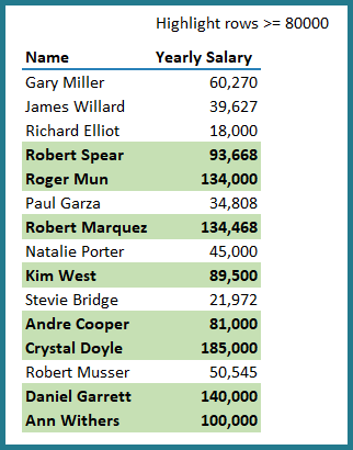
Using a Formula for Conditional Formatting to Highlight a Row
Now that we have the logic nailed down, it’s time to set it up as a Conditional Formatting rule.
❗Remember: We always use the formula created in the UPPER-LEFT corner of the test area.
To update the formula, follow these steps:
- Select the cells with your data (cells A6 to B20).
- Go to the Home tab, find the Styles group, and click on Conditional Formatting. Then, choose New Rule.
- In the New Formatting Rule dialog, pick “Use a formula to determine which cells to format.” Now, enter this formula:
=$B6 > $B$3- Press the “Format” button. This opens the “Format Cells” dialog where you can choose the font color, fill color, and border styles you like.

Click “OK” and get ready to see some impressive results.

Testing the Conditional Formatting Formula
If you change the value in cell B3, the rows matching this new value will automatically update.

Download the Workbook
Feel free to Download the Excel workbook to practice Conditional Formatting to highlight rows HERE.

Leila Gharani
I’ve spent over 20 years helping businesses use data to improve their results. I've worked as an economist and a consultant. I spent 12 years in corporate roles across finance, operations, and IT—managing SAP and Oracle projects.
As a 7-time Microsoft MVP, I have deep knowledge of tools like Excel and Power BI.
I love making complex tech topics easy to understand. There’s nothing better than helping someone realize they can do it themselves. I’m always learning new things too and finding better ways to help others succeed.


