Highlight Max & Min Values in an Excel Line Chart

📥 Learn how to highlight highest and lowest values in Excel charts.

Want to get the most out of this guide? Download the free practice workbook 👉 HERE and follow along.

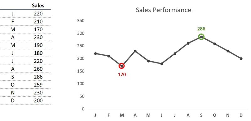
Step 1: Start With a Basic Line Chart

Let’s begin by creating a simple line chart using your data.

1. Click anywhere in your dataset.
2. Go to the Insert tab.
3. In the Charts group, select Insert Line or Area Chart → Line with Markers (top row, second from the right).

What Happens If You Try to Color the Max Value Manually?

If you want to highlight the highest value manually, here’s what you’d do:

• Click once on the line to select the entire series.
• Click a second time on the data point with the highest value to select just that point.
• Right-click the selected data point → choose Format Data Point.
• In the right-hand panel, go to Fill & Line (paint bucket icon).
• Click on Marker, then expand the Fill section.
• Choose a new fill color (e.g. green) for the marker.

The problem?
If your data changes and the highest value moves to a different point, Excel won’t update the color automatically. You’d need to:

• Remove the color from the old point
• Add it to the new one

Step 2: Automatically Highlight Max and Min Points

To make our line chart highlight the highest and lowest values dynamically, we’ll use two helper columns. These will tell Excel which points to color—and update automatically when the data changes.

Create the Helper Columns

We’ll add two new columns to your dataset: one for the MAX value, and one for the MIN value.

1. Next to your original data, add two new headers: MAX and MIN.

2. In the MAX column (e.g., cell C5), enter this formula:

=IF(B5=MAX($B$5:$B$16), B5, ””)

3. In the MIN column (e.g., cell D5), enter this formula:

=IF(B5=MIN($B$5:$B$16), B5, ””)

4. Fill both formulas down for all rows.

Add the MAX and MIN Series to Your Line Chart

Now, let’s add these helper series to the chart.

Method 1: Drag to Expand Data Range

1. Click the edge of your chart to select it.
2. You’ll see a blue border around the data range.
3. Drag the bottom-right handle to include the MAX and MIN columns.

Method 2: Copy & Paste (Alternative)

1. Select the helper data columns, including the headers.
2. Press Ctrl + C to copy.
3. Click the edge of the chart.
4. Press Ctrl + V to paste the series into the chart.

Ignore Zero Values in Excel Chart

Blank cells are plotted as zero on the chart. We will use the NA() function which tells Excel to skip those points completely—no line crashing to the bottom.

1. Select the IF formula for January’s MAX and update it as follows:

=IF(B5=MAX($B$5:$B$16), B5, NA())

2. For the MIN cell of January, update the formula as follows:

=IF(B5=MIN($B$5:$B$16),B5,NA())

3. Fill both formulas down for all rows.

All the “crashed” points have disappeared leaving us with only two additional data points.

Format the Highlight Points

Let’s style the helper series to make them stand out.

1. Click once on the MAX series (e.g., orange point).
   • ❗ Important: Clicking once selects the full series. Clicking twice selects only one point—don’t do that here.

2. Press Ctrl + 1 to open the Format Data Series panel.
   • If you are uncertain if you have the correct series selected, use the Series Options dropdown list to select the proper data series.

3. In the panel, choose the Fill & Line icon (paint bucket).
4. Expand the Marker section:
   • Set marker type to Built-in → Circle
   • Set size to 10

5. Under Fill, choose No Fill

6. Under Border, choose Solid Line
   • Color: Green
   • Width: 2.25 pt

7. Repeat for the MIN series:
   • Same marker and size
   • Border color: Red

Clean Up the Original Line

Let’s simplify the main data series so the highlights pop:

1. Select the Sales series (the original line).
2. In the Format panel:
   • Set marker fill to dark gray
   • Set marker border to none
   • Set line color to dark gray

You can also:

• Make gridlines light gray to soften the background.

Add Data Labels

Want to show the values directly above/below the max and min points?

For the MAX point:

1. Click the MAX series once.
2. Right-click → Add Data Labels
3. Right-click label → Format Data Labels
   • Under Label Options, set Label Position to Above

For the MIN point:

1. Click the MIN series once.
2. Right-click → Add Data Labels
3. Under Label Options, set Label Position to Below

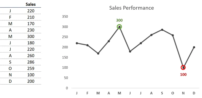
Test It

Try changing a value in your data—for example:

• Set May to 300
• Set November to 100

The highlights will automatically move. No manual updates needed.

Want to Hide the Helper Columns?

You can hide or group the MAX and MIN columns, but by default Excel won’t plot hidden data.

Fix that with these steps:

1. Right-click on the chart → Select Data
2. Click Hidden and Empty Cells (bottom left)
3. Check: Show data in hidden rows and columns

If You Have Duplicate Max or Min Values

You may see a connector line between the duplicate points.

Option 1: Prevent line for hidden columns

• Go to Select Data → Hidden and Empty Cells
• Check: Show #N/A as an empty cell

Option 2: Remove line manually

• Click the series line
• Open Format panel → Fill & Line → Line
• Select: No Line

The result should appear as follows.

Get Creative

This trick doesn’t just work for line charts.

You can use it to:

• Highlight the top bar in a column chart

• Mark the top 3 values in a time series

Download the Free Chat Template

Want to skip the setup and jump right in?

Grab our ready-to-use Excel chart template. It’s pre-built with dynamic highlights for max and min values—so you can start using it right away.

👉 Click here to download the Excel chart template

No formulas to figure out. No formatting needed. Just plug in your data and go.

Featured Bundle

Black Belt Excel Bundle

This Excel Black Belt Package includes EIGHT of our Popular Courses. You’ll learn high-value, in-depth Excel skills that solve real problems.

Learn More

LinkedIn Twitter YouTube

Leila Gharani

I’ve spent over 20 years helping businesses use data to improve their results. I've worked as an economist and a consultant. I spent 12 years in corporate roles across finance, operations, and IT—managing SAP and Oracle projects.

As a 7-time Microsoft MVP, I have deep knowledge of tools like Excel and Power BI.

I love making complex tech topics easy to understand. There’s nothing better than helping someone realize they can do it themselves. I’m always learning new things too and finding better ways to help others succeed.

More About Leila Join 400,000+ professionals in our courses